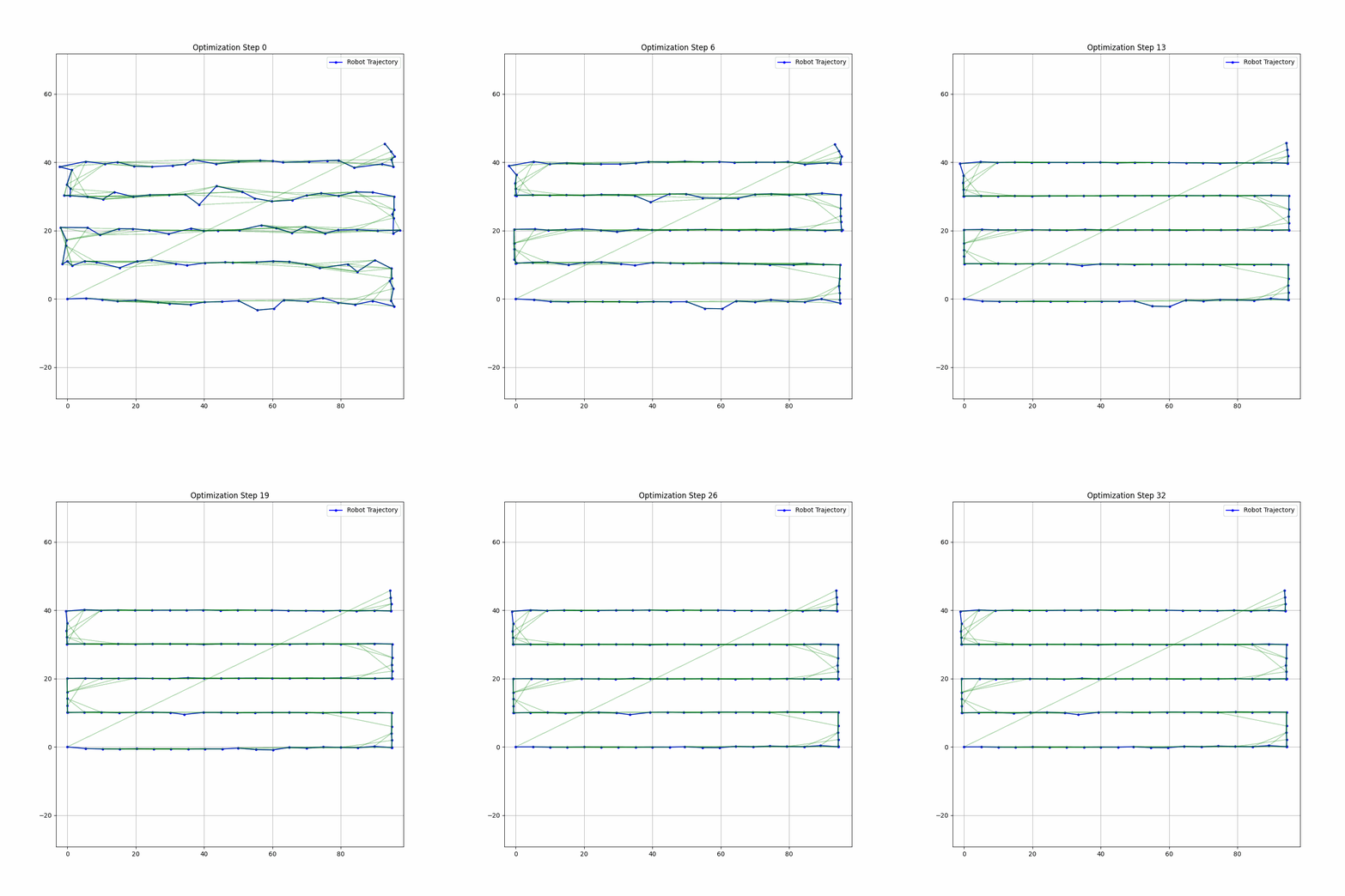
Graph SLAM is a cornerstone technique in modern robotics that elegantly solves the simultaneous localization and mapping problem through graph optimization. This comprehensive tutorial covers everything from theoretical foundations to practical implementation, making it suitable for both learning and reference.
Introduction
The SLAM Problem

Simultaneous Localization and Mapping (SLAM) addresses two fundamental questions in robotics:
- Where is the robot in the environment? (Localization)
- What does the environment look like? (Mapping)
These questions are inherently interconnected:
- Accurate mapping requires precise localization
- Precise localization requires an accurate map
- This chicken-and-egg problem makes SLAM challenging
Graph SLAM Overview
Graph SLAM approaches this challenge by:
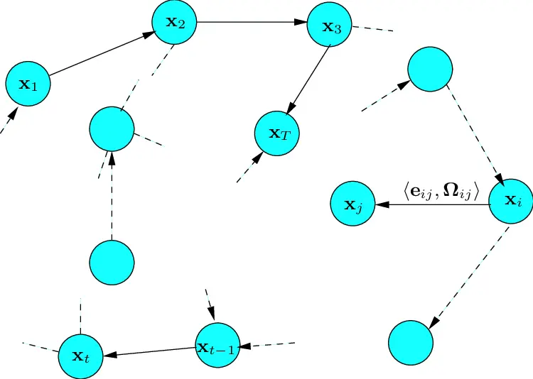
- Representing the problem as a graph optimization task
- Modeling robot poses and landmarks as nodes
- Representing measurements and constraints as edges
- Using optimization techniques to find the most consistent solution
Theoretical Foundation
1. Graph-Based Formulation
Graph SLAM represents the SLAM problem using a graph structure where:
Nodes Represent:
- Robot poses at different timestamps (position and orientation)
- Landmarks or features observed in the environment
- Environmental structure points or objects
Edges Represent:
- Odometry measurements between consecutive poses
- Sensor observations of landmarks from different poses
- Loop closure constraints when revisiting areas
- Relative transformations between poses
| Graph Element | Real-world Meaning | Mathematical Representation |
|---|---|---|
| Pose Node | Robot's position and orientation at time t | x_t = (x, y, θ) in 2D |
| Landmark Node | Static feature in environment | m_i = (x, y) in 2D |
| Odometry Edge | Robot movement measurement | u_t = (Δx, Δy, Δθ) |
| Observation Edge | Landmark measurement from pose | z_t = (r, φ) (range, bearing) |
Frontend and Backend SLAM
Graph SLAM consists of two main components:
-
Frontend: Responsible for data association and loop closure detection
- Sensor Data Processing: Handles raw sensor data from sources such as LIDAR, cameras, and IMUs.
- Feature Extraction: Identifies and extracts significant features or landmarks from the sensor data.
- Data Association: Matches observed features with previously seen landmarks to establish correspondences.
- Loop Closure Detection: Identifies when the robot revisits a previously mapped area, crucial for correcting accumulated drift.
- Graph Construction: Creates nodes (representing robot poses and landmarks) and edges (representing constraints) in the graph.
-
Backend: Handles optimization of the graph
- Graph Optimization: Takes the graph structure as input and optimizes the poses and landmarks to minimize the overall error.
- Error Minimization: Uses techniques like Gauss-Newton or Levenberg-Marquardt to iteratively reduce the error in the graph.
- Covariance Estimation: Estimates the uncertainty associated with each pose and landmark, providing a measure of confidence.
- Sparse Matrix Operations: Efficiently handles large-scale optimization problems using sparse matrix representations.
The frontend processes raw data and builds the graph, while the backend optimizes it. This separation allows for modularity, enabling different implementations for each component based on specific requirements and sensor configurations. The frontend ensures accurate data association and loop closure detection, while the backend focuses on refining the map and trajectory through robust optimization techniques.
2. Key Components
Graph Representation
class GraphSLAM:
    def __init__(self):
        self.poses = []          # Robot pose nodes
        self.landmarks = []      # Landmark nodes
        self.odom_edges = []     # Odometry constraints
        self.obs_edges = []      # Observation constraints
        self.loop_edges = []     # Loop closure constraints
Motion Model
The motion model is used to predict the robot's next pose based on its current pose and control inputs. It is essential for estimating the robot's trajectory over time.
Inputs:
- Previous pose estimate (position and orientation)
- Control inputs (e.g., velocity, angular velocity) or odometry measurements (e.g. wheel encoders, measured velocity...)
- Time interval (duration of the control input)
Outputs:
- Predicted next pose (position and orientation)
Generic Formulation: The motion model can be represented as a function that takes the previous pose , control input , and time interval to produce the next pose :
The function typically accounts for the robot's kinematics and/or dynamics to predict the next pose accurately.
One example of a motion model for a differential drive robot is:
where:
- is the previous pose
- are the linear and angular velocities
- is the time interval
def predict_motion(prev_pose: Pose2D, control: Control) -> Pose2D:
    """
    Predict next pose based on control input and motion model
    """
    dx = control.velocity * math.cos(prev_pose.theta) * control.dt
    dy = control.velocity * math.sin(prev_pose.theta) * control.dt
    dtheta = control.angular_velocity * control.dt

    return Pose2D(
        x=prev_pose.x + dx,
        y=prev_pose.y + dy,
        theta=prev_pose.theta + dtheta
    )
Sensor Model
The sensor model is used to predict the expected measurements (e.g. range and bearing) from the robot's sensors given its current state and the positions of landmarks. It is essential for comparing predicted measurements with actual sensor readings to update the robot's belief about its environment.
Inputs:
- Current pose estimate (position and orientation)
- Landmark position (e.g., coordinates of a feature in the environment)
Outputs:
- Predicted measurement (e.g., range and bearing to the landmark)
Generic Formulation: The sensor model can be represented as a function that takes the current pose and the landmark position to produce the predicted measurement :
The function typically accounts for the geometry of the sensor and the relative position of the landmark to the robot.
One example of a sensor model for a range-bearing sensor is:
where:
- is the current pose
- is the landmark position
Error Function
In the context of graph-based SLAM (Simultaneous Localization and Mapping), the error function is used to quantify the difference between predicted and actual measurements or transformations. This is crucial for optimizing the pose graph to minimize these differences, leading to a more accurate map and better localization.
Why We Need the Error Function
The error function is essential because it allows us to:
- Quantify Discrepancies: Measure how far off our predictions are from the actual measurements.
- Optimize the Graph: Use optimization techniques to adjust the poses and minimize the error, improving the overall accuracy of the SLAM system.
Mathematical Formula
The error function for a given edge in the pose graph can be defined as:
-
For odometry edges:
where
-
For observation edges:
where is the landmark index observed from pose and is the index of the observation from pose to landmark
Example in Code
Here's a simplified example in Python to illustrate how you might define an error function in a graph-based SLAM system:
def compute_error(pred: Measurement, actual: Measurement,
                 information: np.ndarray) -> float:
    """
    Compute weighted error between predicted and actual measurements
    """
    error = pred - actual
    return error.T @ information @ error
Mathematical Formulation
Problem Definition
The Graph SLAM optimization problem aims to estimate the robot's trajectory and the map based on noisy odometry and observation measurements.
Given:
- Odometry measurements between consecutive robot poses
- Observation measurements of landmarks from robot pose
- Motion model , where represents motion noise
- Observation model , where represents observation noise
Where:
- is the robot's pose at time
- represents the th landmark's position in the map
- is the control input (odometry measurement) from time to
- is the observation of landmark from pose
- and are functions representing the motion and observation models respectively
Optimization Problem
Graph SLAM seeks to find the maximum a posteriori (MAP) estimate for the trajectory and landmarks :
Using Bayes' theorem and assuming independence of noise:
Negative Log Likelihood
The problem can be transformed into minimizing the negative log-likelihood:
where:
- represents a weighted Mahalanobis distance
- is the covariance matrix of the motion noise
- is the covariance matrix of the observation noise
Components of the Objective Function
-
Odometry Term:
- Penalizes differences between predicted and actual poses
- Encodes consistency between consecutive poses using odometry data
-
Observation Term:
- Measures discrepancy between observed and expected measurements
- Ensures landmarks match predicted observations
Final Mathematical Formulation
The complete objective function to minimize is:
Optimization Strategies
The optimization problem is often solved using iterative nonlinear optimization techniques such as:
- Gauss-Newton Method or Levenberg-Marquardt algorithms for nonlinear least squares (unconstrained optimization).
- Graph-based approaches that use sparse matrix representations for large-scale SLAM problems.
Linearization and Gauss-Newton Method
To solve the nonlinear optimization problem posed by Graph SLAM using the Gauss-Newton method, we first need to linearize the problem around an initial estimate and iteratively refine the solution. Here is the step-by-step formulation of the linearization and solution using Gauss-Newton.
Linearization of the Problem
To apply the Gauss-Newton method, we linearize the nonlinear functions and using a first-order Taylor expansion around the current estimate and . Denote the current estimate as for robot poses and for landmark positions.
a. Motion Model Linearization
Given the motion model residual:
linearize around and :
where:
are the Jacobians of the motion model.
b. Observation Model Linearization
Given the observation model residual:
linearize around and :
where:
are the Jacobians of the observation model.
Linearized Least-Squares Problem
Substitute these linearized residuals into the original cost function to form a quadratic approximation:
This is a linear least-squares problem, which can be written in matrix form as:
where:
- is a sparse matrix composed of the Jacobians and .
- is a vector composed of the negative residuals and weighted by the information matrices.
Gauss-Newton Iterative Update
Solve for the increment by solving the linear system:
Update the current estimates:
Repeat this process until the change in the objective function is below a predefined threshold or the increment becomes sufficiently small.
Convergence and Implementation Notes
- The method assumes that the Jacobians and are recomputed at each iteration.
- The matrix is often sparse, allowing for efficient solutions using techniques like sparse Cholesky decomposition.
- The Gauss-Newton method works well when the initial guess is close to the optimal solution. For large errors or highly nonlinear problems, additional techniques like Levenberg-Marquardt may be used for better convergence.
Step-by-Step Process:
- Initialize with odometry-based estimate
- For each iteration:
- Compute errors for all constraints
- Linearize around current estimate
- Solve linear system
- Update poses and landmarks
- Continue until convergence
class GraphOptimizer:
    def optimize(self, max_iterations: int = 100,
                convergence_thresh: float = 1e-6) -> None:
        """
        Optimize the pose graph using Gauss-Newton method
        """
        for iteration in range(max_iterations):
            # Compute total error
            prev_error = self.compute_total_error()

            # Build linear system
            H = np.zeros((self.state_dim, self.state_dim))
            b = np.zeros(self.state_dim)

            # Add constraints
            self.add_pose_constraints(H, b)
            self.add_landmark_constraints(H, b)
            self.add_loop_closure_constraints(H, b)

            # Solve system
            dx = np.linalg.solve(H, -b)

            # Update poses and landmarks
            self.update_state(dx)

            # Check convergence
            current_error = self.compute_total_error()
            if abs(prev_error - current_error) < convergence_thresh:
                break
Implementation Deep Dive
Implementation details
The following example will solve a simplified Graph Optimization problem where:
- Robot poses are represented as 2D poses (x, y)
- There are no landmark observations
- Only odometry constraints are considered, in order to estimate robot trajectory multiple odometry measurements are used for between nodes, usually a not realistic scenario but for simplicity, we will consider this.
1. Core Data Structures
Pose Representation
@dataclass
class Pose2D:
    """Represents a 2D robot pose (x, y, θ)"""
    x: float
    y: float
    theta: float = 0.0

    def to_matrix(self) -> np.ndarray:
        """Convert to homogeneous transformation matrix"""
        c = math.cos(self.theta)
        s = math.sin(self.theta)
        return np.array([
            [c, -s, self.x],
            [s,  c, self.y],
            [0,  0,    1]
        ])

    def inverse(self) -> 'Pose2D':
        """Compute inverse transformation"""
        c = math.cos(self.theta)
        s = math.sin(self.theta)
        x = -c * self.x - s * self.y
        y =  s * self.x - c * self.y
        return Pose2D(x, y, -self.theta)
Graph Structure
class PoseGraph:
    def __init__(self):
        self.nodes: List[Pose2D] = []
        self.edges: List[Edge] = []
        self.covariances: Dict[int, np.ndarray] = {}

    def add_node(self, pose: Pose2D,
                 covariance: Optional[np.ndarray] = None) -> int:
        """Add a new node to the graph"""
        node_id = len(self.nodes)
        self.nodes.append(pose)
        if covariance is not None:
            self.covariances[node_id] = covariance
        return node_id

    def add_edge(self, from_id: int, to_id: int,
                 measurement: Pose2D,
                 information: np.ndarray) -> None:
        """Add a new edge (constraint) to the graph"""
        edge = Edge(from_id, to_id, measurement, information)
        self.edges.append(edge)
2. Graph Construction
Building the Graph
class GraphBuilder:
    def __init__(self):
        self.pose_graph = PoseGraph()
        self.current_pose_id = None

    def add_odometry_measurement(self,
                               odom_measurement: Pose2D,
                               uncertainty: np.ndarray) -> None:
        """Add new pose and odometry edge to graph"""
        # Create new pose node
        new_pose = self.predict_new_pose(odom_measurement)
        new_pose_id = self.pose_graph.add_node(new_pose)

        # Add odometry edge if not first pose
        if self.current_pose_id is not None:
            information = np.linalg.inv(uncertainty)
            self.pose_graph.add_edge(
                self.current_pose_id,
                new_pose_id,
                odom_measurement,
                information
            )

        self.current_pose_id = new_pose_id

    def add_landmark_observation(self,
                               landmark_id: int,
                               measurement: Measurement,
                               uncertainty: np.ndarray) -> None:
        """Add landmark observation edge"""
        information = np.linalg.inv(uncertainty)
        self.pose_graph.add_edge(
            self.current_pose_id,
            landmark_id,
            measurement,
            information,
            edge_type="observation"
        )
3. Loop Closure Detection
Loop closure is crucial for correcting accumulated drift:
class LoopClosureDetector:
    def __init__(self, pose_graph: PoseGraph,
                 distance_threshold: float = 2.0,
                 similarity_threshold: float = 0.75):
        self.pose_graph = pose_graph
        self.distance_threshold = distance_threshold
        self.similarity_threshold = similarity_threshold
        self.descriptor_database = []

    def detect_loop_closures(self,
                           current_pose: Pose2D,
                           current_scan: LaserScan,
                           current_descriptor: np.ndarray) -> List[LoopClosure]:
        """Detect potential loop closures"""
        loop_closures = []

        # Find nearby poses
        nearby_poses = self.find_nearby_poses(current_pose)

        for pose_id, pose in nearby_poses:
            # Skip recent poses
            if abs(pose_id - len(self.pose_graph.nodes) + 1) < 50:
                continue

            # Check scan similarity
            if self.check_scan_similarity(current_scan,
                                       self.descriptor_database[pose_id],
                                       current_descriptor):
                # Compute relative transform
                transform = self.compute_relative_transform(
                    current_pose, pose)

                # Verify geometric consistency
                if self.verify_geometric_consistency(transform):
                    loop_closures.append(
                        LoopClosure(pose_id, transform))

        return loop_closures

    def check_scan_similarity(self,
                            current_scan: LaserScan,
                            stored_scan: LaserScan,
                            current_descriptor: np.ndarray) -> bool:
        """Check if two laser scans are similar"""
        score = self.compute_descriptor_similarity(
            current_descriptor,
            self.descriptor_database[stored_scan.id]
        )
        return score > self.similarity_threshold
4. Advanced Optimization Techniques
Sparse Matrix Optimization
class SparseGraphOptimizer:
    def __init__(self, pose_graph: PoseGraph):
        self.pose_graph = pose_graph

    def build_sparse_system(self) -> Tuple[sparse.csr_matrix, np.ndarray]:
        """Build sparse linear system for optimization"""
        rows, cols, data = [], [], []
        b = np.zeros(self.state_dimension)

        for edge in self.pose_graph.edges:
            # Compute Jacobians
            J_i, J_j = self.compute_edge_jacobians(edge)

            # Add to sparse system
            omega = edge.information
            H_ii = J_i.T @ omega @ J_i
            H_ij = J_i.T @ omega @ J_j
            H_jj = J_j.T @ omega @ J_j

            # Update sparse matrices
            self.update_sparse_matrices(
                rows, cols, data,
                edge.from_id, edge.to_id,
                H_ii, H_ij, H_jj
            )

            # Update right-hand side
            error = self.compute_edge_error(edge)
            b[self.index_mapping(edge.from_id)] += J_i.T @ omega @ error
            b[self.index_mapping(edge.to_id)] += J_j.T @ omega @ error

        H = sparse.csr_matrix((data, (rows, cols)))
        return H, b
5. Robust Error Functions
class RobustKernel:
    def huber_loss(self, error: np.ndarray, delta: float) -> Tuple[float, float]:
        """
        Implement Huber loss function for robust optimization
        Returns (weighted_error, weight)
        """
        error_norm = np.linalg.norm(error)

        if error_norm <= delta:
            # Quadratic region
            return error_norm**2, 1.0
        else:
            # Linear region
            return 2 * delta * error_norm - delta**2, delta / error_norm

class RobustGraphOptimizer(GraphOptimizer):
    def __init__(self, pose_graph: PoseGraph, kernel: RobustKernel):
        super().__init__(pose_graph)
        self.kernel = kernel

    def compute_weighted_error(self, edge: Edge) -> np.ndarray:
        """Compute error with robust weighting"""
        error = self.compute_edge_error(edge)
        _, weight = self.kernel.huber_loss(error, delta=1.0)
        return error * weight
6. Real-world Applications and Optimizations
Dynamic Environment Handling
class DynamicSLAM(GraphSLAM):
    def __init__(self):
        super().__init__()
        self.dynamic_object_detector = DynamicObjectDetector()
        self.static_map = OccupancyGrid()

    def process_scan(self, scan: LaserScan) -> None:
        """Process laser scan considering dynamic objects"""
        # Detect and remove dynamic objects
        static_scan = self.dynamic_object_detector.filter_dynamic_objects(scan)

        # Update static map
        self.static_map.update(static_scan)

        # Add to pose graph with increased uncertainty for dynamic regions
        uncertainty = self.compute_adaptive_uncertainty(scan)
        self.add_scan_to_graph(static_scan, uncertainty)
Multi-robot SLAM
class MultiRobotSLAM:
    def __init__(self, robot_count: int):
        self.robots = [GraphSLAM() for _ in range(robot_count)]
        self.relative_poses = {}
        self.shared_landmarks = {}

    def merge_maps(self) -> None:
        """Merge individual robot maps"""
        for i in range(len(self.robots)):
            for j in range(i + 1, len(self.robots)):
                # Find common landmarks
                common = self.find_common_landmarks(
                    self.robots[i], self.robots[j])

                if len(common) >= 3:
                    # Compute relative transformation
                    transform = self.compute_relative_transform(
                        self.robots[i], self.robots[j], common)

                    # Merge pose graphs
                    self.merge_pose_graphs(i, j, transform)
7. Visualization and Analysis
class SLAMVisualizer:
    def __init__(self, pose_graph: PoseGraph):
        self.pose_graph = pose_graph
        self.fig, self.ax = plt.subplots(figsize=(12, 8))

    def visualize_graph(self) -> None:
        """Visualize current state of pose graph"""
        self.ax.clear()

        # Plot poses
        poses = np.array([[pose.x, pose.y] for pose in self.pose_graph.nodes])
        self.ax.plot(poses[:, 0], poses[:, 1], 'b.-', label='Robot Path')

        # Plot edges
        for edge in self.pose_graph.edges:
            if edge.type == "odometry":
                color = 'g'
            elif edge.type == "loop_closure":
                color = 'r'
            else:
                color = 'y'

            self.plot_edge(edge, color)

        # Plot uncertainty ellipses
        self.plot_uncertainty_ellipses()

        plt.legend()
        plt.axis('equal')
        plt.draw()

    def plot_uncertainty_ellipses(self) -> None:
        """Plot uncertainty ellipses for poses"""
        for node_id, covariance in self.pose_graph.covariances.items():
            pose = self.pose_graph.nodes[node_id]
            eigenvals, eigenvecs = np.linalg.eig(covariance[:2, :2])
            angle = np.arctan2(eigenvecs[1, 0], eigenvecs[0, 0])

            ellip = patches.Ellipse(
                (pose.x, pose.y),
                2 * np.sqrt(eigenvals[0]),
                2 * np.sqrt(eigenvals[1]),
                angle=np.degrees(angle),
                fill=False,
                color='gray',
                alpha=0.3
            )
            self.ax.add_patch(ellip)
8. Performance Optimization
class OptimizedGraphSLAM:
    def __init__(self):
        self.pose_graph = PoseGraph()
        self.node_cache = LRUCache(1000)
        self.kdtree = None

    def update_spatial_index(self) -> None:
        """Update KD-tree for spatial queries"""
        poses = np.array([[pose.x, pose.y] for pose in self.pose_graph.nodes])
        self.kdtree = spatial.cKDTree(poses)

    def find_nearby_poses(self,
                         query_pose: Pose2D,
                         radius: float) -> List[int]:
        """Find poses within radius using KD-tree"""
        if self.kdtree is None:
            self.update_spatial_index()

        query_point = np.array([query_pose.x, query_pose.y])
        indices = self.kdtree.query_ball_point(query_point, radius)
        return indices
Best Practices and Tips
-
Loop Closure
- Implement conservative loop closure detection
- Use multiple validation steps
- Consider appearance and geometric consistency
-
Optimization
- Use sparse matrix operations
- Implement robust error functions
- Consider incremental optimization for real-time applications
-
Performance
- Implement node pruning for long-term operation
- Use spatial indexing for neighbor searches
- Consider parallel processing for large graphs
Conclusion
Graph SLAM provides a powerful framework for solving the SLAM problem by:
- Representing the problem as an optimization task
- Handling uncertainty through probabilistic frameworks
- Correcting accumulated errors through loop closures
- Providing a flexible foundation for extensions
Future directions include:
- Integration with deep learning methods
- Improved dynamic environment handling
- Enhanced semantic mapping capabilities
- Real-time performance optimizations
References and Further Reading
- Grisetti, G., Kummerle, R., Stachniss, C., & Burgard, W. (2010). "A Tutorial on Graph-Based SLAM"
- Dellaert, F., & Kaess, M. (2006). "Square Root SAM"
- Stachniss, C., Leonard, J., & Thrun, S. (2016). "Simultaneous Localization and Mapping"
- Kaess, M., Johannsson, H., Roberts, R., Ila, V., Leonard, J., & Dellaert, F. (2012). "iSAM2: Incremental Smoothing and Mapping Using the Bayes Tree"
- Cadena, C., Carlone, L., Carrillo, H., Latif, Y., Scaramuzza, D., Neira, J., Reid, I., & Leonard, J. J. (2016). "Past, Present, and Future of Simultaneous Localization and Mapping: Toward the Robust-Perception Age"
- Thrun, S., & Montemerlo, M. (2006). "The GraphSLAM Algorithm with Applications to Large-Scale Mapping of Urban Structures"


