Wake-Word Detection for your AI robot: A Step-by-Step Guide

Wake-Word Detection for your AI robot: Step-by-Step Guide

In this guide, we will walk you through the process of building a wake word detection system for Argo, an AI home robot. Along the way, we will also highlight the general pipeline used in AI projects, making this guide perfect for those new to Artificial Intelligence (AI), Natural Language Processing (NLP), or robotics.

Watch the full video of Argo on YouTube!

Throughout the development, we’ll focus on the following stages:

1. Dataset Creation: Learn how to gather and prepare high-quality data for training your model.
2. Dataset Augmentation: Discover techniques to expand and diversify the dataset, enhancing model robustness.
3. Feature Selection: Understand how to extract the most relevant features from raw data to boost performance.
4. Neural Network Architecture: Learn how to design a model capable of effectively learning patterns from the data.
5. Training and Evaluation: Gain insights into optimizing and evaluating the model to ensure it performs at its best.
6. Deployment: Understand the steps for preparing the model for integration into real-world applications.

By following this structured approach, you will not only learn how to build a wake word detection system but also gain a solid framework for tackling a wide range of AI challenges. Whether you’re a student, hobbyist, or aspiring professional, this guide will equip you with the skills and knowledge to begin your journey into AI and robotics.

1. Problem Overview

Argo is an home robot designed for autonomous navigation, conversational AI, entertainment, and much more. As a companion robot, it is essential for Argo to recognize when it is called by its owner, making wake word detection a critical skill. The goal is for Argo to detect the phrase "Hey Argo" reliably, while ignoring background noise or irrelevant speech. Once detected, Argo will quickly switch into attention mode to respond appropriately.

This task relies on a technique called supervised learning. The concept is simple: by showing a machine multiple examples of labeled data, such as images of cats and dogs with the corresponding labels, the system learns to recognize patterns. Similarly, by feeding the model audio files containing (or not) the wake word "Hey Argo", it will learn to differentiate between when the wake word is spoken and when it is not.

2. Dataset Creation

So the first step in AI taks is to gather a vast dataset of examples from which our model can learn from. For our dataset, we basically recorded two types of audio:

• "positive" samples: 300 recordings of people saying "Hey Argo".

• "negative" samples: 500 recordings of random noise, silence or other words.

Below is a simple script to record 3-seconds audio samples and save them as .wav files with the corresponding label (positive or negative) embedded in the filename.

import pyaudio
import wave

def record_audio(filename, duration=3, fs=16000):

    p = pyaudio.PyAudio()
    stream = p.open(format=pyaudio.paInt16, channels=1, rate=fs, input=True)

    # Read audio data in a single shot
    print(f"Recording {filename}...")
    data = stream.read(int(fs * duration))  
    print("Finished recording.")

    # stop stream
    stream.stop_stream()
    stream.close()
    p.terminate()

    # save audio in .wav
    with wave.open(filename, 'wb') as wf:
        wf.setnchannels(1)
        wf.setsampwidth(p.get_sample_size(pyaudio.paInt16))
        wf.setframerate(fs)
        wf.writeframes(data)

# Example usage
record_audio("positive_sample_01.wav")

3. Dataset Augmentation

Data augmentation is essential for building a robust wake word detection system. It enhances the model's generalization by simulating real-world conditions such as background noise, pitch variations, and different speaking speeds. By expanding the dataset with augmented samples, the model becomes more resilient to variations in speakers, accents, and environments, ensuring reliable performance in diverse scenarios.

Moreover, collecting and labeling real-world audio data can be both time-consuming and costly. Imagine the challenge of recording diverse audio samples from hundreds of different people with various voices. Data augmentation helps mitigate the need for extensive data collection. Instead of recording new audio, we can generate additional data by applying various transformations to existing recordings. These transformations allow us to effectively expand our dataset without the need for new recordings. Below are some of the transformations we can apply to each audio sample:

1. Pitch shifting
2. Audio stretching
3. Random noise

Below is a script to perform data augmentation:

import librosa

def pitch_shift(audio_path, output_path, shift):

    # Apply pitch shifting to audio file
    y, sr = librosa.load(audio_path, sr=None) 
    y_shifted = librosa.effects.pitch_shift(y, sr, shift)  
    sf.write(output_path, y_shifted, sr)

def stretch_audio(audio_path, output_path, rate):

    # Stretch or compress the audio duration
    y, sr = librosa.load(audio_path, sr=None) 
    y_stretched = librosa.effects.time_stretch(y, rate)  
    sf.write(output_path, y_stretched, sr) 

def add_noise(audio_path, output_path, noise_factor=0.005):

    # Add random noise to the audio file to simulate background interference
    y, sr = librosa.load(audio_path, sr=None)
    noise_amp = noise_factor * np.random.uniform() * np.amax(y)  
    y_noisy = y + noise_amp * np.random.normal(size=y.shape) 
    sf.write(output_path, y_noisy, sr)

4. Feature Selection: Mel-Spectrogram

Feature selection is a crucial step in building machine learning models, especially when working with audio data. The goal of feature extraction is to transform raw audio into a more compact and informative representation, making it easier for models to learn patterns and make predictions. In our case, we chose the Mel-Spectrogram as the primary feature representation of the audio signal. This method converts the audio signal into the frequency domain, breaking it down into its spectral components (how much energy exists at various frequencies).

Given an input audio file, its raw format is typically represented as a one-dimensional array 1 x N , where:

• N: The number of time steps or samples in the audio file.
• 1: Each value in the array represents the audio intensity (amplitude) at a specific time step.

After applying a spectrogram transformation, the audio data is converted into a 2D representation with dimensions M x K, where:

• K: The number of time frames (total_number_of_samples / hop_length)
• M: It corresponds to the range of frequencies in the signal (n_mels).

Thus, instead of being represented by a single value at each time step, the audio is now represented by a richer vector with n_mels elements, capturing more detailed information about the frequency content at each time frame.

Code to compute the Mel-spectrogram:

from torchaudio import transforms
import matplotlib.pyplot as plt

def spectro_gram(aud, n_mels=64, n_fft=1024, hop_len=None):

    # Load the audio signal
    sig, sr = aud  # 'sig' is the audio signal, 'sr' is the sampling rate
    
    # The threshold in decibels for filtering weak signals
    top_db = 80  
    
    # Apply MelSpectrogram transformation
    spec = transforms.MelSpectrogram(sample_rate=sr, n_fft=n_fft, hop_length=hop_len, n_mels=n_mels)(sig)
    
    # Convert amplitude to decibels (logarithmic scale)
    spec = transforms.AmplitudeToDB(top_db=top_db)(spec)
    
    return spec  # Shape: [n_mels, time_steps]

5. Neural Network Architecture

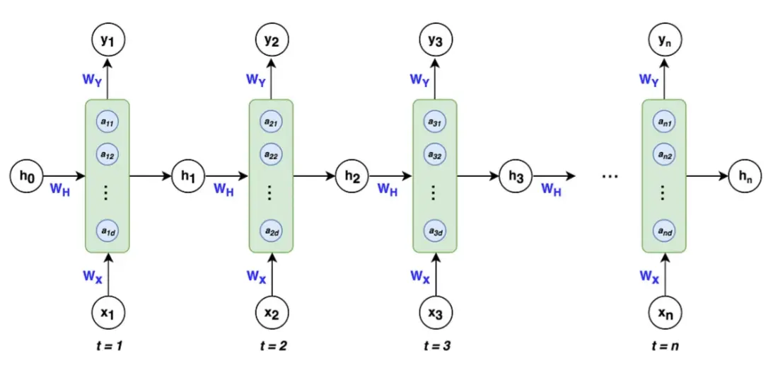
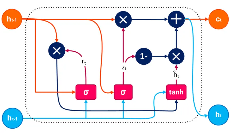
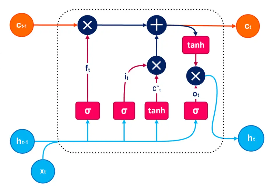
We analyzed three main architectures: RNN, GRU, and LSTM. Below is a brief theoretical description and the code for each.

RNN (Recurrent Neural Network)

Recurrent Neural Networks (RNNs) calculate temporal representations by processing sequences one timestep at a time using a recurrent mechanism. The basic equation is:

Where:

• $h_t$: Hidden state at time $t$ with dimensions $(sequence\_length \times hidden\_size)$
• $x_t$: Input vector at time $t$ with dimensions $(sequence\_length \times input\_size)$
• $h_{t-1}$: Hidden state from the previous timestep with dimensions $(sequence\_length \times hidden\_size)$
• $W_h$, $U_h$: Weight matrices
• $b_h$: Bias vector

import torch
import torch.nn as nn

class RNNModel(nn.Module):
    
    def __init__(self, input_size, hidden_size, output_size, num_layers):
        super(RNNModel, self).__init__()
        self.rnn = nn.RNN(input_size, hidden_size, num_layers, batch_first=True) 
        self.fc = nn.Linear(hidden_size, output_size)
    
    
    def forward(self, x):
        # input: batch_size, sequence_length, features --> output: batch_size, sequence_length, hidden_size
        out, _ = self.rnn(x) 
        # input: batch_size, hidden_size --> output: batch_size, output_size
        out = self.fc(out[:, -1, :]) 
        return out

# net hyperparameters
batch_size=32
epochs=120
learning_rate=0.00005 
input_size = 64 # n_mels 
hidden_size = 256
output_size = 1  # Output size for binary classification
num_layers = 2

# define the model
model = RNNModel(input_size, hidden_size, output_size, num_layers)

Using the Last Hidden State for Classification:

In classification tasks, instead of using the entire sequence of hidden states, we often use only the hidden state from the final timestep ($h_{T}$). This state serves as a compact representation of the entire input sequence, containing the most relevant information for the task. To perform classification, the final hidden state is passed through a Fully Connected (FC) layer. The FC layer has an output dimension of $1$, producing a scalar value that represents the probability of the audio belonging to a specific class ("positive" or "negative").

GRU (Gated Recurrent Unit)

Gated Recurrent Units (GRUs) improve upon standard RNNs by introducing gating mechanisms that regulate the flow of information. The GRU has two main gates: the update gate and the reset gate. The key equations are:

Where:

• $h_t$: Hidden state at time $t$ with dimensions $(sequence\_length \times hidden\_size)$
• $x_t$: Input vector at time $t$ with dimensions $(sequence\_length \times input\_size)$
• $\tilde{h}_t$: Candidate hidden state with dimensions $(sequence\_length \times hidden\_size)$
• $z_t$, $r_t$: Update and reset gates
• $W_z$, $W_r$, $W_h$: Weight matrices for input features
• $U_z$, $U_r$, $U_h$: Weight matrices for hidden state
• $b_z$, $b_r$, $b_h$: Bias vectors
• $\sigma$: Sigmoid activation function
• $\odot$: Element-wise multiplication

class GRUModel(nn.Module):
    
    def __init__(self, input_size, hidden_size, output_size, num_layers):
        super(GRUModel, self).__init__()
        self.gru = nn.GRU(input_size, hidden_size, num_layers, batch_first=True)
        self.fc = nn.Linear(hidden_size, output_size)
    
    def forward(self, x):
        out, _ = self.gru(x)
        out = self.fc(out[:, -1, :])
        return out

# net hyperparameters
batch_size=32
epochs=100
learning_rate=0.0001   
input_size = 64 # n_mels
hidden_size = 256*2
output_size = 1  # Output size for binary classification
num_layers = 1

# define the model
model = GRUModel(input_size, hidden_size, output_size, num_layers)

LSTM (Long Short-Term Memory)

Long Short-Term Memory Networks (LSTMs) are an advanced type of RNN designed to handle long-term dependencies in sequential data. They use a set of gates to control the flow of information: the forget gate, input gate, and output gate, as well as a cell state to store long-term memory. The key equations for LSTM are:

Where:

• $h_t$: Hidden state at time $t$ with dimensions $(sequence\_length \times hidden\_size)$
• $c_t$: Cell state at time $t$ with dimensions $(sequence\_length \times hidden\_size)$
• $\tilde{c}_t$: Candidate cell state with dimensions $(sequence\_length \times hidden\_size)$
• $x_t$: Input vector at time $t$ with dimensions $(sequence\_length \times input\_size)$
• $f_t$, $i_t$, $o_t$: Forget, input and output gates with dimensions $(sequence\_length \times hidden\_size)$
• $W_f$, $W_i$, $W_c$, $W_o$: Weight matrices for input features
• $U_f$, $U_i$, $U_c$, $U_o$: Weight matrices for hidden state
• $b_f$, $b_i$, $b_c$, $b_o$: Bias vectors
• $\sigma$: Sigmoid activation function
• $\tanh$: Hyperbolic tangent activation function
• $\odot$: Element-wise multiplication

LSTM Workflow:

• The cell state ($c_t$) acts as long-term memory, modified by the forget and input gates.
• The hidden state ($h_t$) acts as the short-term output, determined by the output gate and the updated cell state.

class LSTMModel(nn.Module):
    
    def __init__(self, input_size, hidden_size, output_size, num_layers):
        super(LSTMModel, self).__init__()
        self.lstm = nn.LSTM(input_size, hidden_size, num_layers, batch_first=True)
        self.fc = nn.Linear(hidden_size, output_size)
    
    def forward(self, x):
        out, _ = self.lstm(x)
        out = self.fc(out[:, -1, :])
        return out

# net hyperparameters
batch_size = 32
epochs = 50
learning_rate = 0.0001
input_size = 64 # n_mels 
hidden_size = 256 * 2
output_size = 1  # Output size for binary classification
num_layers = 1

# define model
model = LSTMModel(input_size, hidden_size, output_size, num_layers)

6. Training and Evaluation

Training is the process of optimizing the model’s parameters (weights and biases) so it can learn to make predictions. To achieve this, the dataset is divided into two parts:

• Training set (80%): Used to train the model by adjusting its weights to minimize the error.
• Validation set (20%): Used to evaluate the model's performance after training, to check how well it generalizes to unseen data.

    # Random split of 80:20 between training and validation
    num_items = len(dataset)
    num_train = round(num_items * 0.8)
    num_val = num_items - num_train
    train_ds, val_ds = random_split(dataset, [num_train, num_val])
    print("train set: ", num_train)
    print("valid set: ", num_val)

During training, the model learns by minimizing a loss function, which quantifies the error between the predicted and actual labels. For this binary classification task, we use Binary Cross-Entropy with Logits Loss (BCEWithLogitsLoss):

Where:

• $z_i$: Raw logits from the model
• $\sigma(z_i)$: Sigmoid function converting logits to probabilities
• $y_i$: True label (0 or 1)
• $N$: Batch size

During training, a gradient descent algorithm is used to change iteratively the model's weights and minimize the loss. Main steps:

1. Compute gradients of the loss $\nabla L$ w.r.t. the weights.
2. Update weights: $w_{new} = w_{old} - \eta \cdot \nabla L$

Where $\eta$ is the learning rate and $\nabla L$ is the gradient of the loss.

Throughout training, we monitor the average loss at the end of each epoch. A decreasing training loss indicates that the model is learning. Once training is complete, we save the learned weights to be used for deployment.

# Using BCEWithLogitsLoss
criterion = nn.BCEWithLogitsLoss()
optimizer = optim.Adam(model.parameters(), lr=learning_rate)

def train_model(train_dl):
    
    # For plotting
    train_loss_values = []

    # Training loop
    for epoch in range(epochs):
        
        model.train()
        epoch_loss = 0
        
        for i, (inputs, labels) in enumerate(train_dl):

            # inference
            outputs = model(inputs)
            
            # compute loss
            loss = criterion(outputs, labels)
            optimizer.zero_grad()
            loss.backward()
            optimizer.step()
            
            epoch_loss += loss.item()

        # check loss after each epoch
        average_loss = epoch_loss / len(train_dl)
        train_loss_values.append(average_loss)
        print(f'Epoch [{epoch+1}/{epochs}], Loss: {average_loss:.4f}')

    # save final model weights
    torch.save(model.state_dict(), "model_weights")

    # Plot loss
    plt.plot(range(1, epochs + 1), train_loss_values, marker='o')
    plt.title('Training Loss')
    plt.xlabel('Epoch')
    plt.ylabel('Loss')
    plt.grid(True)
    plt.show()

Finally, we validate the model using the validation set. This step involves loading the saved weights and evaluating the model’s performance on unseen data using metrics such as accuracy or precision. Validation ensures that the model's performance generalizes to real-world scenarios.

# Using BCE With LogitsLoss 
criterion = nn.BCEWithLogitsLoss()
optimizer = optim.Adam(model.parameters(), lr=learning_rate)

# Load model weights
model.load_state_dict(torch.load('model_weights.pth'))

def eval_model(val_dl):
    
    model.eval()
    valid_loss = 0
    all_labels = []
    all_predictions = []

    with torch.no_grad():
        
        # Loop through validation set
        for inputs, labels in val_dl:
            
            # Inference
            outputs = model(inputs)

            # Compute loss as metrics
            loss = criterion(outputs, labels)
            valid_loss += loss.item()
            
            # Calculate predictions
            predicted_probs = torch.sigmoid(outputs)
            predicted_labels = (predicted_probs >= 0.5).float()
            
            # Store labels and predictions for metric calculation
            all_labels.extend(labels.numpy()) 
            all_predictions.extend(predicted_labels.numpy()) 

    # Calculate accuracy
    accuracy = accuracy_score(all_labels, all_predictions)

7. Deployment

In this final step, we deploy the trained wake word detection model to a real-time system. The goal is to continuously process audio data, extract features, and evaluate the model to detect if the wake word "Hey Argo" is spoken. The deployment involves handling live audio streams, computing spectrograms, and passing the extracted features to the neural network for inference.

Below, a callback function processes audio in chunks, maintains a rolling buffer of audio samples, and prepares the data for feature extraction. This ensures that the neural network always receives the latest audio segment for evaluation.

def callback(in_data, frame_count, time_info, status): 
    
    global run, data 

    # Transform audio bytes to a numpy array
    new_data = np.frombuffer(in_data, dtype='int16')
    
    # Update the rolling buffer: dequeue oldest samples and enqueue the latest
    data = np.roll(data, -chunk_samples) 
    data[feed_samples - chunk_samples:] = new_data[:] 
    
    # Store the updated buffer in the queue
    que.put(data)
    
    return (in_data, pyaudio.paContinue)

The main script initializes the audio stream, processes audio chunks, extracts features, and evaluates the model. It continuously listens for the wake word and prints results in real-time.

# audio stream parameters
fs=16000 # sample rate
chunk_duration = 1.0 # each read window
feed_duration = 2.944   # the total feed length (the actual input for the NN)
chunk_samples = int(fs * chunk_duration) 
feed_samples = int(fs * feed_duration)

if __name__ == '__main__':

    print('Start recording...')

    # Set up a queue and data buffer
    que = Queue() 
    data = np.zeros(feed_samples, dtype='int16')  # Rolling buffer for audio input
    run = True

    # Initialize PyAudio
    p = pyaudio.PyAudio()

    # Set up and start the audio stream
    stream = p.open(format=pyaudio.paInt16,
                    channels=1,  # Mono audio
                    rate=fs,  # Sample rate
                    input=True,
                    frames_per_buffer=chunk_samples,  # Chunk size in samples
                    stream_callback=callback)
    
    stream.start_stream()
    
    try:
        while run:
            # Retrieve the latest audio segment
            data = que.get()
                      
            # Extract features (spectrogram)
            sgram = spectro_gram((data, fs))
            
            # Evaluate the model
            is_wake_word_detected = eval_model(sgram)
            
            # Display the result
            if is_wake_word_detected:
                print("Hey Argo detected!")
            else:
                print("Random word")
            
    except (KeyboardInterrupt, SystemExit):
        print("Exiting... Bye.")
        run = False

    # Clean up resources
    stream.stop_stream()
    stream.close()
    p.terminate()

The model is finally ready to be executed on your laptop.. or on your Argo if you have one!

8. Directories & Code

On git-hub, you can find a full implementation of the aforementioned wake-word detection system. The directories are organized in the following way:

Code

• build_dataset.py: code used to create the dataset and augment (eventually) the dataset.
• audio_processing_lib.py: this code contains the functions related to audio processing (record, compute spectrogram, ..).
• dataset_processing_lib.py: this code contains the functions related to dataset processing (create and augment dataset, get dataloader, ..).
• nn_architecture.py: code defining different NN architectures.
• wake_word_training.py: code for training.
• wake_word_eval.py: code for running inference over a singli input audio file.
• wake_word_live.py: code for recording audio live and print the wake word when it is detected.
• dynamic_quantization.py: code for applying dynamic quantization to the saved model (model_weights.ph), so as to have faster and lighter inference on embedded devices.

Dataset

• originals: positive words "Hey Argo" and negative words (random words or background noise).
• augemented: takes the file in "originals" and augment them with pitch shifting and audio stretching.

Models

Weights of the NN trained on different datasets (augmented vs orginals) and different architectures (RNN, GRU, LSTM).

9. Key Works and Citations

• Graves et al. (2013): Speech Recognition with Deep Recurrent Neural Networks.
• Andrew Ng. (Coursera): Deep Learning Specialization: Sequence Models.