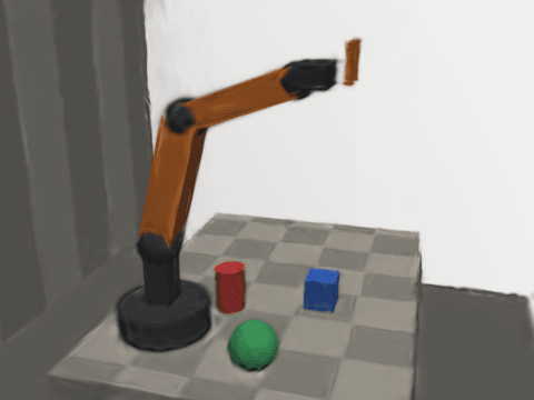
A robot needs a representation of the world it is about to act in. Historically we have picked from a short menu: point clouds, occupancy grids, TSDFs, meshes, and more recently neural fields. Each choice encodes an assumption about what the robot will do with the world — plan through it, collide with it, localize in it, or learn from it.
3D Gaussian Splatting (3DGS) adds an unusual option: represent the scene as a few million semi-transparent ellipsoids, and optimize them until rendering those ellipsoids from your camera poses reproduces your photographs. The result is not a surface. It is closer to a photographic volume — one you can render from new viewpoints at hundreds of frames per second.
This post is about how that actually works, starting from the representation and
ending at the rasterizer. The visuals are generated from a real training run on a
synthetic robot workcell — a 6-DOF arm with a parallel gripper, a checkerboard
table, and a cube/ball/can — ray-traced from 60 known camera poses (200×150
px). The 60 images are rendered with a custom ray tracer
(synthetic_scene.py)
that also outputs the exact camera-to-world transforms and a set of initial 3D
points sampled from the scene surface. Because the poses are known analytically,
no COLMAP, SfM, or external pose estimator was involved. Every Gaussian center,
every covariance, and every colour is learned directly from those 60 images plus
their poses.
1. Why not a mesh, a voxel grid, or a NeRF?
Every scene representation makes a trade.
Voxels are trivial to reason about and trivial to collide with, but memory grows cubically with resolution. A workcell at millimetre resolution is a lot of empty air stored as zeros.
Meshes are the native language of physics engines and planners, but recovering topology from images is hard, thin structures are miserable, and a single albedo texture cannot represent the sheen on an aluminium extrusion.
NeRFs represent the scene as a neural network queried along each ray. They are compact and beautifully smooth, but rendering means evaluating a network hundreds of times per pixel, and training means millions of such evaluations.
Gaussian splatting makes a different bet: don't learn a function, learn the primitives themselves. Put a few million explicit, differentiable blobs in space and optimize their parameters directly with gradient descent. Because the primitives are explicit, rendering can be a fast, sorted, tile-based rasterizer instead of a per-pixel network query.
The price is that the scene is not a surface. It is a cloud of soft ellipsoids with no topology, no watertightness, and no notion of "inside". We will come back to why that matters for robots.
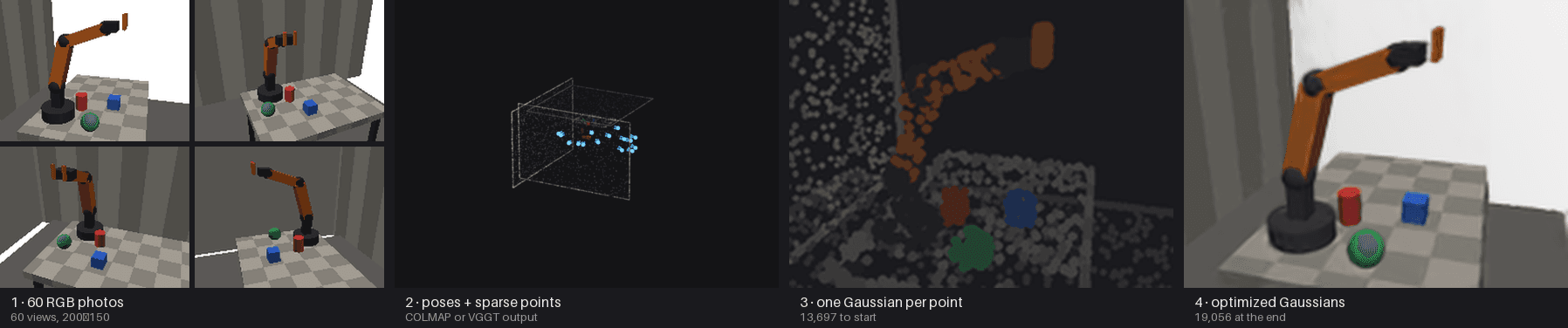
The pipeline in one picture: the 60 input photographs, the camera poses they came from, the sparse cloud that initialises the Gaussians, and — after a few thousand gradient steps — the dense field of Gaussians that reproduces the scene. In this demo, the poses and the initial point cloud come from the ray tracer, not from COLMAP or a pose estimator. The data inputs are exactly the 60 images plus their camera-to-world transforms; no additional scanning, feature matching, or manual calibration was needed.
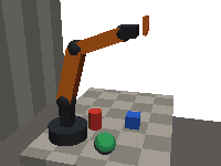
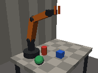
Here are three of the 60 input images at different viewpoints — the arm, gripper, table, cube, ball, and can visible from various angles:

2. Anatomy of one Gaussian
Each Gaussian is defined by four groups of parameters:
- Position : where the blob sits.
- Covariance : its shape and orientation, factored into a rotation quaternion and a diagonal scale . This is what lets one Gaussian be a flat pancake on a table, a needle along a cable, or a sphere on a ball joint.
- Opacity : how much light it blocks.
- Colour : spherical-harmonic coefficients, so colour can change with viewing direction.
The covariance factorization is the important design choice. Optimizing a full covariance directly would be unconstrained and could easily become non-positive-definite. Optimizing a scale and a quaternion keeps symmetric positive semi-definite by construction, and gives the optimizer parameters with intuitive meaning.
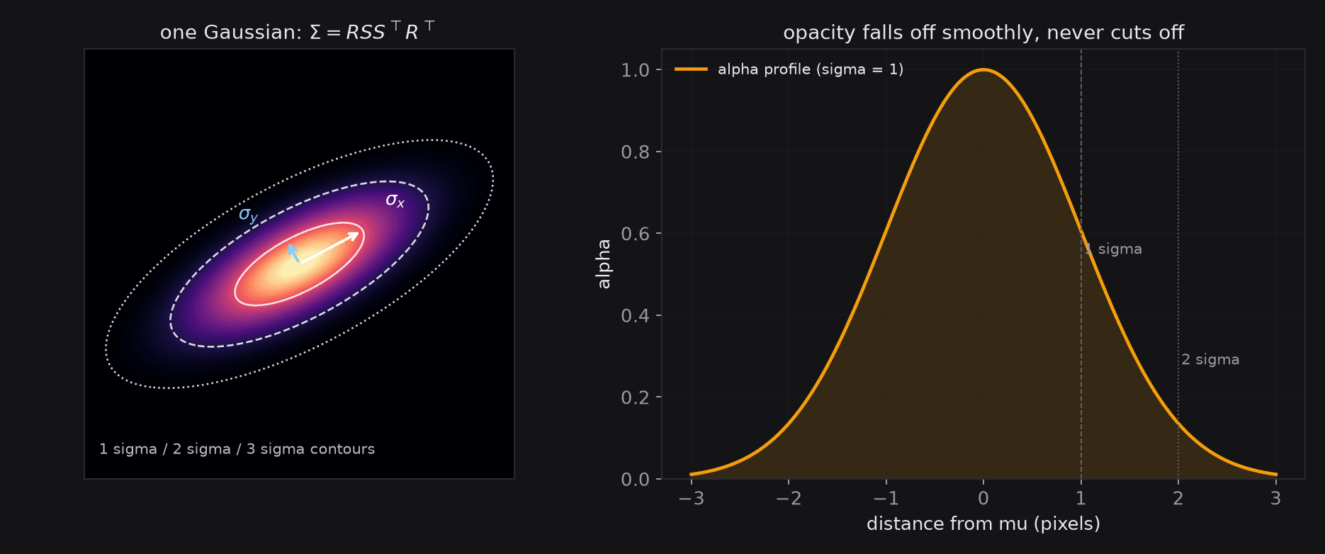
A Gaussian never "ends" at its edge. Its alpha decays smoothly, which is exactly what makes overlapping blobs composite into a continuous surface instead of a pointillist mess. In practice the rasterizer ignores contributions beyond three standard deviations, but that is a performance cut, not a modelling one.
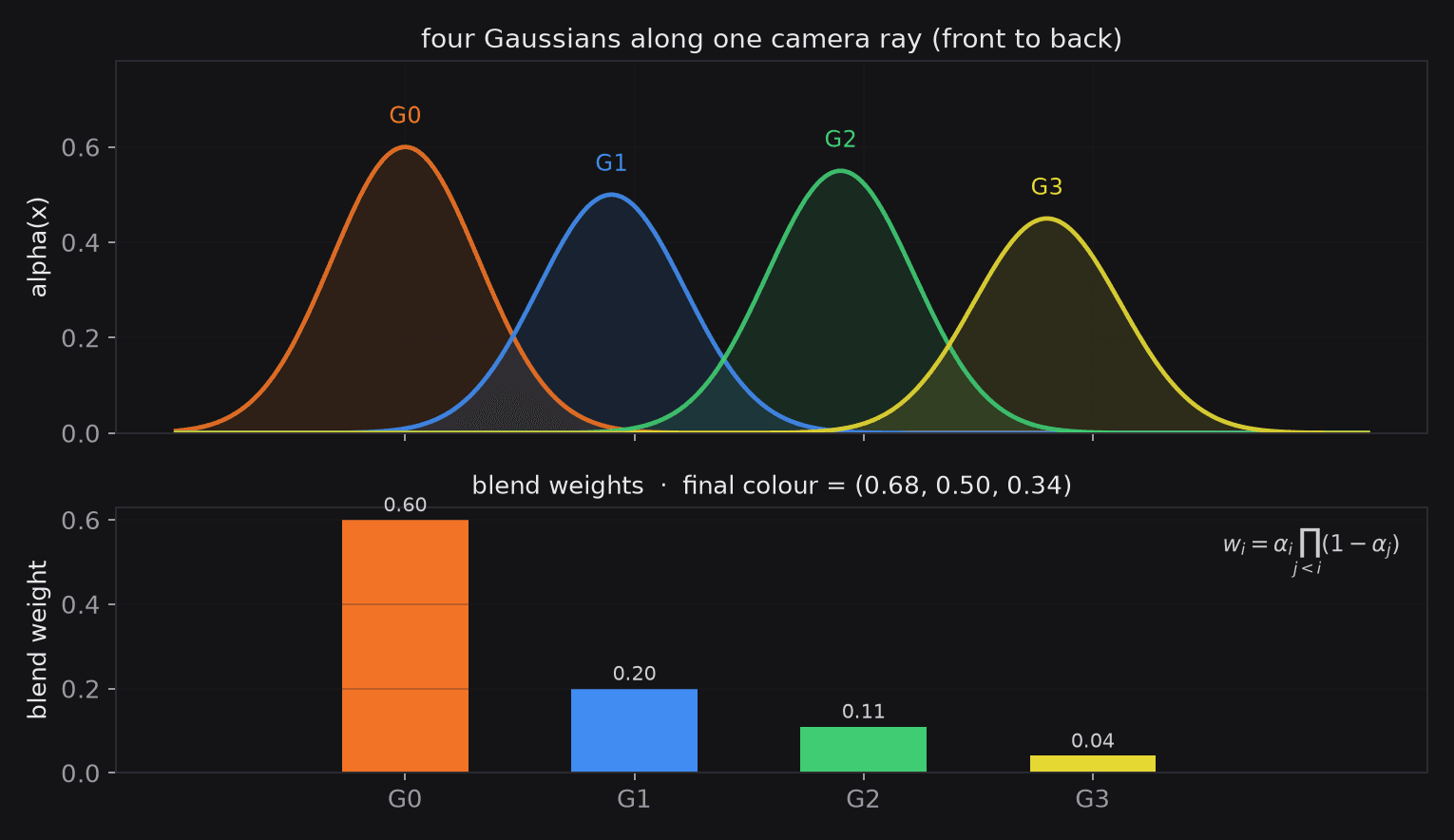
At a pixel covered by all three, each weight is αᵢ · Π(1−αⱼ) for the Gaussians in front of it. Pull a Gaussian to zero opacity and watch the ones behind it reappear.
The lab above is the whole representation in miniature: shape is covariance, opacity is alpha, and the final pixel is a weighted sum, not a maximum or an average. Pull one Gaussian's opacity to zero and the ones behind it reappear — that is the compositing equation doing its job.
Why spherical harmonics?
A single RGB value is view-independent: the blob looks the same from every angle. Real surfaces are not like that. Brushed metal, glossy plastic, and polycarbonate guards all change appearance with viewing direction.
Spherical harmonics are a smooth basis on the sphere. Storing a few coefficients per colour channel lets the network of Gaussians approximate that angular dependence. Degree 0 is a constant colour; degree 3 stores 16 coefficients per channel and captures most specular effects you can see in a workcell.
Degree 0 is not a downgrade for many robotics uses. It is smaller, faster, and more stable under novel viewpoints. Use degree 3 when reflections are part of what you need to reproduce.
3. From 3D blobs to 2D pixels
To render, each 3D Gaussian has to become a 2D Gaussian on the image plane. The naive approach — project the center, then reuse the 3D scale — is wrong: a Gaussian seen edge-on should look thin, and one seen face-on should look wide. Perspective also changes apparent size with depth.
The standard answer is the EWA approximation (Zwicker et al., 2002): locally linearize the perspective projection and push the covariance through its Jacobian.
where is the world-to-camera rotation and
evaluated at the Gaussian's center in camera space. This is the same first-order approximation you would use for any uncertainty propagation: the projection is nonlinear, but over the footprint of one Gaussian it is approximately affine.
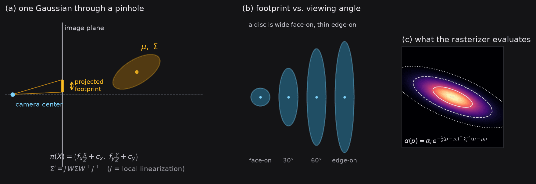
The diagram above unpacks the projection in three ways: (a) a single Gaussian viewed from the side, with tangent rays tracing its image-plane footprint; (b) the same covariance seen from different angles — face-on is wide, edge-on is thin; (c) the resulting 2D Gaussian that the rasterizer actually evaluates with the conic equation.
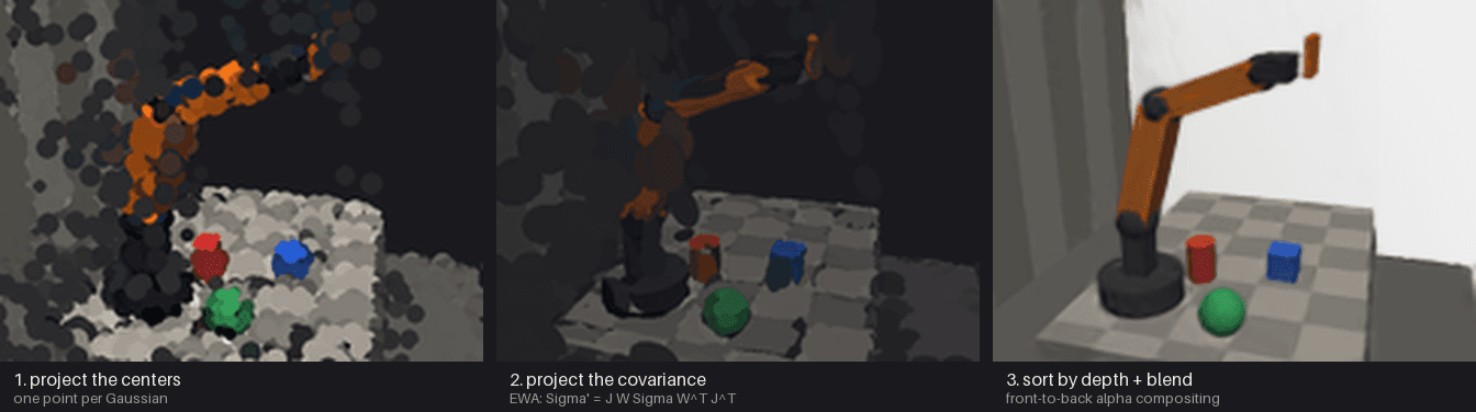
The figure above is the pipeline on real data: first the centers, then the projected 2-sigma ellipses, then the blended image. The ellipses are not decoration — they are the rasterizer's input. Each one becomes a quadratic form (a "conic"), so evaluating a Gaussian at a pixel is a handful of multiply-adds:
The inverse covariance is precomputed per Gaussian per frame. Everything after that is embarrassingly parallel, which is why this renders in real time.
4. Sorting and compositing
Gaussians overlap, so the renderer must decide what is in front. It sorts by depth and composites front-to-back:
Each Gaussian's contribution is attenuated by everything in front of it. This is the same over-operator used in alpha compositing everywhere, just applied to thousands of primitives per pixel.
Sorting is also the method's structural weakness. It is global per frame (or per tile in optimized implementations), it is not differentiable, and it has to be redone whenever the camera moves. A misplaced Gaussian can pop in front of another between frames — one reason splats shimmer under fast motion.
The original implementation sorts with a custom CUDA radix sort and renders 16×16 tiles. The from-scratch version in this post does the same thing in PyTorch: sort once per frame, then composite per tile. Same math, orders of magnitude slower.
5. Learning the scene
Training is analysis-by-synthesis. Pick a camera, render the current Gaussians from it, compare with the real photo, and backpropagate the error into every parameter. Repeat a few thousand times.
The loss is a combination of per-pixel and structural error:
L1 keeps colours honest; SSIM discourages blurry, low-contrast solutions. Adam updates all parameters, but not at the same rate: position moves slowly (), colour and opacity move faster, and the position learning rate is decayed exponentially so the geometry settles instead of jittering.
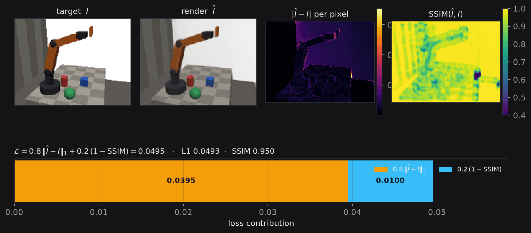
The loss decomposition above shows the signal the optimizer actually sees: the target and render side by side, the per-pixel L1 difference, the SSIM map (a value near 1.0 means the local patch is well reconstructed), and the two loss terms stacked into a bar chart. The SSIM term penalises blurry regions where L1 alone would let the optimizer settle for a smooth average.
Where do the Gaussians start?
They start from structure-from-motion points. COLMAP matches features across images, solves camera poses, and triangulates a sparse cloud. One Gaussian is placed per point, with colour from the point and scale from the mean distance to its neighbours.
This is not a detail. SfM points land on actual surfaces, which gives the optimizer both a sane position and a sane scale. Random initialization in a bounding box mostly produces fog.
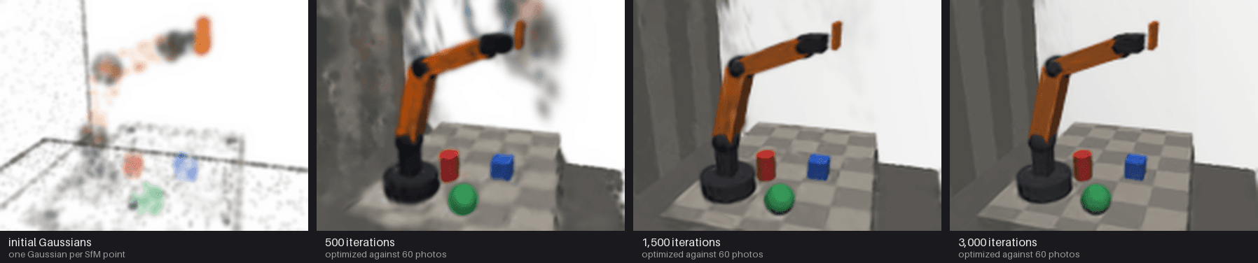
Early iterations mostly fix colour and opacity; geometry sharpens later. By the end, the arm and the checkerboard are coherent, while thin structures (gripper fingers, cables) remain the softest part of the reconstruction — they occupy too few pixels to constrain well.
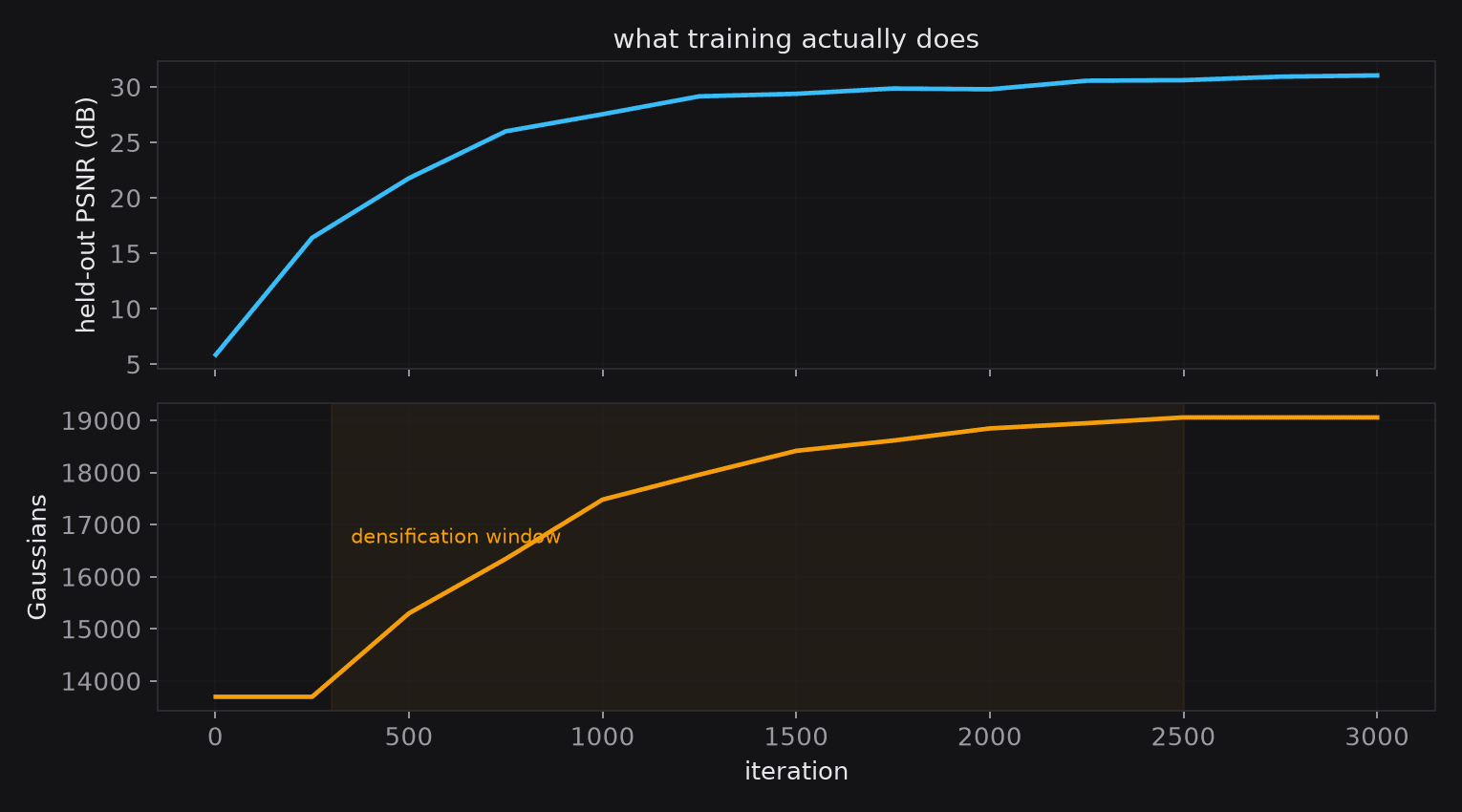
The held-out PSNR is measured on cameras excluded from training, so it is an honest check that the model generalizes to new viewpoints rather than memorizing the input frames.
6. Where new Gaussians come from
A fixed set of SfM points cannot represent both a flat table and a thin finger. So the optimizer edits its own model during training:
- Clone small Gaussians in regions with a large image-space gradient.
- Split large Gaussians in those regions into two smaller ones, sampled from the original distribution.
- Prune Gaussians whose opacity has decayed below a threshold.
The trigger is the magnitude of the gradient flowing back to the projected center: high error in a region means "put more capacity here". The size of the Gaussian decides whether to clone (it is already small; duplicate it) or split (it is too coarse; subdivide it).
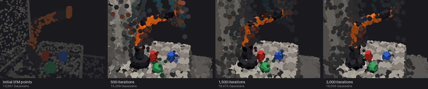
The placement figure is the part I find most instructive. Densification is not uniform: capacity piles up on edges, texture, and thin geometry, and stays sparse on flat, low-gradient surfaces. That is the method allocating its budget where the loss says it matters.
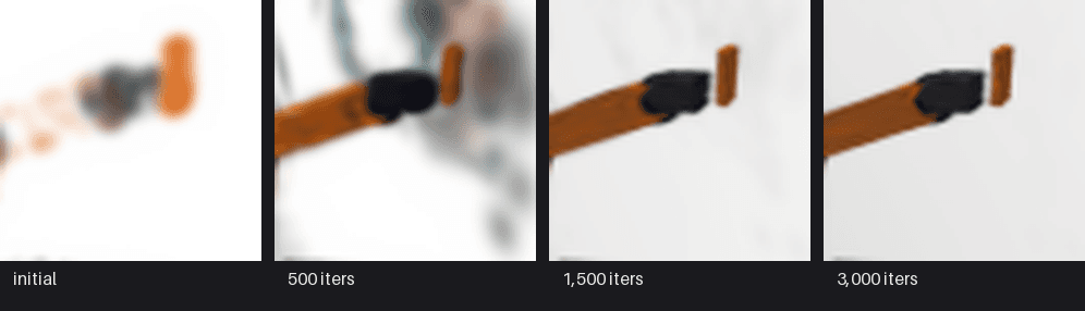
Densification is also the main cost driver. More Gaussians mean more memory, more sorting, and bigger files. The practical knobs — gradient threshold, split threshold, the clone/split size rule, maximum count — are all dials on that trade.
7. What the result looks like
Here is the final model, with 19,056 Gaussians trained on 60 views. Drag it around; the point is not that it is perfect, but that it is a scene you can interrogate from angles that were never photographed.
Preparing splats…
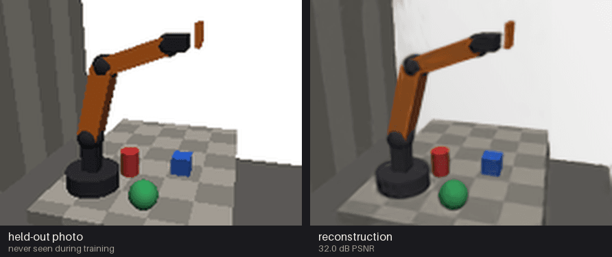
The comparison above is the honest test: a camera that was never in the training set, rendered from the optimized Gaussians. It lands at 32.0 dB held-out PSNR. The geometry holds up; the photometry is slightly softer than the original, and the thin gripper fingers are the first thing to blur.
8. The part robotics makes hard: poses
Everything above assumes you know where each photo was taken. In a lab, that is the step that decides whether the project works.
COLMAP is the default. It needs 30–100 images with strong overlap, and it will fail quietly on textureless surfaces, motion blur, or repetitive structure. A workcell full of white plastic and aluminium is not an easy SfM scene.
Few-view estimators (VGGT, MASt3R, DUSt3R) predict poses and dense geometry directly from images, without classical feature matching. They make 5–15 photo captures possible, which is attractive for quick robot-cell scans. But be honest about the trade: with five views you are fitting a radiance field to five directions. Orbit away from them and the Gaussians stretch into floating soup. Few-view 3DGS is an active research area, not a solved workflow.
Practical capture rules that save hours:
- 70–85% overlap between consecutive frames.
- No motion blur; it corrupts both poses and radiance.
- Lock exposure and white balance. Auto-exposure gets baked into the Gaussians as a brightness gradient across the scene.
- Keep the scene static. A moved object becomes a ghost with two positions.
- For a workcell, capture it empty and populated if both matter.
And one robotics-specific trap: monocular capture has a global scale ambiguity. The reconstruction does not know whether the table is 60 cm or 6 m wide. If you need metric scale, you need a calibrated stereo rig, a known reference object, or an additional sensor.
9. What this buys a roboticist
Photoreal data engines. Render a real workcell from new camera poses to augment demonstrations for imitation-learning policies, without rebuilding the cell in a simulator. The visual gap to reality shrinks, and with it part of the sim-to-real gap.
Digital twins. Reconstruct once, then inspect, plan, or onboard remotely. Because rendering is real-time, the twin can live in a browser or a headset.
Dense mapping. Systems like SplaTAM and GS-SLAM use Gaussians as the map itself, optimizing photometrically while tracking the camera. The appeal is a map that is both geometrically dense and renderable — useful for relocalization and for human operators.
Sim-to-real backdrops. A splat is a cheap photoreal environment for synthetic data. It is not a physics representation: no contacts, no friction, no dynamics.
10. Where it breaks
- It is not a mesh. Gaussians are soft and non-manifold. For grasping and collision checking you still want a surface. Methods like 2DGS and SuGaR extract one, but that is a separate step with its own failure modes.
- It is not dynamic. A splat is a snapshot. Moving grippers and manipulated objects smear unless time is modelled explicitly.
- It is not scale-aware. See above.
- It is not small. Millions of Gaussians mean hundreds of megabytes, and streaming them to a robot or a browser is its own engineering problem.
- It is not robust to lighting changes. The scene learns the illumination it was captured under.
Most of these are active research areas, which is exactly why the field is interesting right now.
References & Further Reading
Foundation
- 3D Gaussian Splatting for Real-Time Radiance Field Rendering — Kerbl, Kopanas, Leimkühler, Drettakis, SIGGRAPH 2023. The paper that started it: differentiable 3D Gaussians, tile-based rasterization, and the densification strategy this article builds on.
- EWA Splatting — Zwicker, Pfister, van Baar, Gross, IEEE TVCG 2002. The original EWA volume-splatting framework: locally linearize perspective, push covariance through the Jacobian — everything Section 3 uses.
- A Comprehensive Overview of Gaussian Splatting — Yurkova, Towards Data Science, 2023. A clear step-by-step walkthrough of the representation, rendering, and optimization.
SLAM & dense mapping
- SplaTAM: Splat, Track & Map 3D Gaussians for Dense RGB-D SLAM — Keetha et al., CVPR 2024. Gaussian splatting used as the dense map in a real-time SLAM system; tracking and mapping in a single differentiable representation.
- GS-SLAM: Dense Visual SLAM with 3D Gaussian Splatting — Yan et al., CVPR 2024. The first RGB-D SLAM system built entirely on 3D Gaussian primitives, with adaptive expansion and coarse-to-fine tracking.
- Gaussian-SLAM: Photo-realistic Dense SLAM with Gaussian Splatting — Yugay et al., 2023. Extends Gaussians to large-scale scenes via submap-based online optimization.
Geometric extensions
- 2D Gaussian Splatting for Geometrically Accurate Radiance Fields — Huang et al., SIGGRAPH 2024. Flattens 3D Gaussians into 2D discs so the radiance field has a well-defined surface — useful when you need normals or collision geometry.
- SuGaR: Surface-Aligned Gaussian Splatting for Efficient 3D Mesh Reconstruction — Guédon & Lepetit, CVPR 2024. Regularises Gaussians to lie on surfaces, then extracts a mesh via Poisson reconstruction — one of the first reliable mesh-from-splat pipelines.
Pose estimation & few-view reconstruction
- COLMAP: Structure-from-Motion Revisited — Schönberger & Frahm, CVPR 2016. The standard SfM/MVS pipeline; still the de-facto pose-estimation front-end for 3DGS.
- VGGT: Visual Geometry Grounded Transformer — Wang et al., CVPR 2025. Feed-forward network that regresses camera parameters, point maps, and depth from one or a few views — no feature matching needed.
- DUSt3R: Geometric 3D Vision Made Easy — Wang et al., CVPR 2024. Regresses dense pointmaps directly from unposed image pairs; the base model for MASt3R.
- MASt3R: Grounding Image Matching in 3D — Leroy et al., ECCV 2024. Augments DUSt3R with a matching head for accurate correspondences at extreme viewpoint changes.